6.1 Discrete and continuous time models

The mathematical analyses presented in Chapters 1 through 5 are based on the assumption that system behavior can be characterized  by a trajectory such as the one shown in Figure 6-1.   In graphs of this type, the vertical axis represents a set of observable states and the horizontal axis represents a time-ordered sequence of transition points.  These transition points represent the only times at which a change of state can occur

For the discrete time processes discussed in Chapters 1 through 5, the only information available at each transition point is the new state that has just been entered.  [It is possible for the  new state to be the same as the current state.] Each transition point and its associated “new state” are represented in Figure 6-1 by a separate black dot.

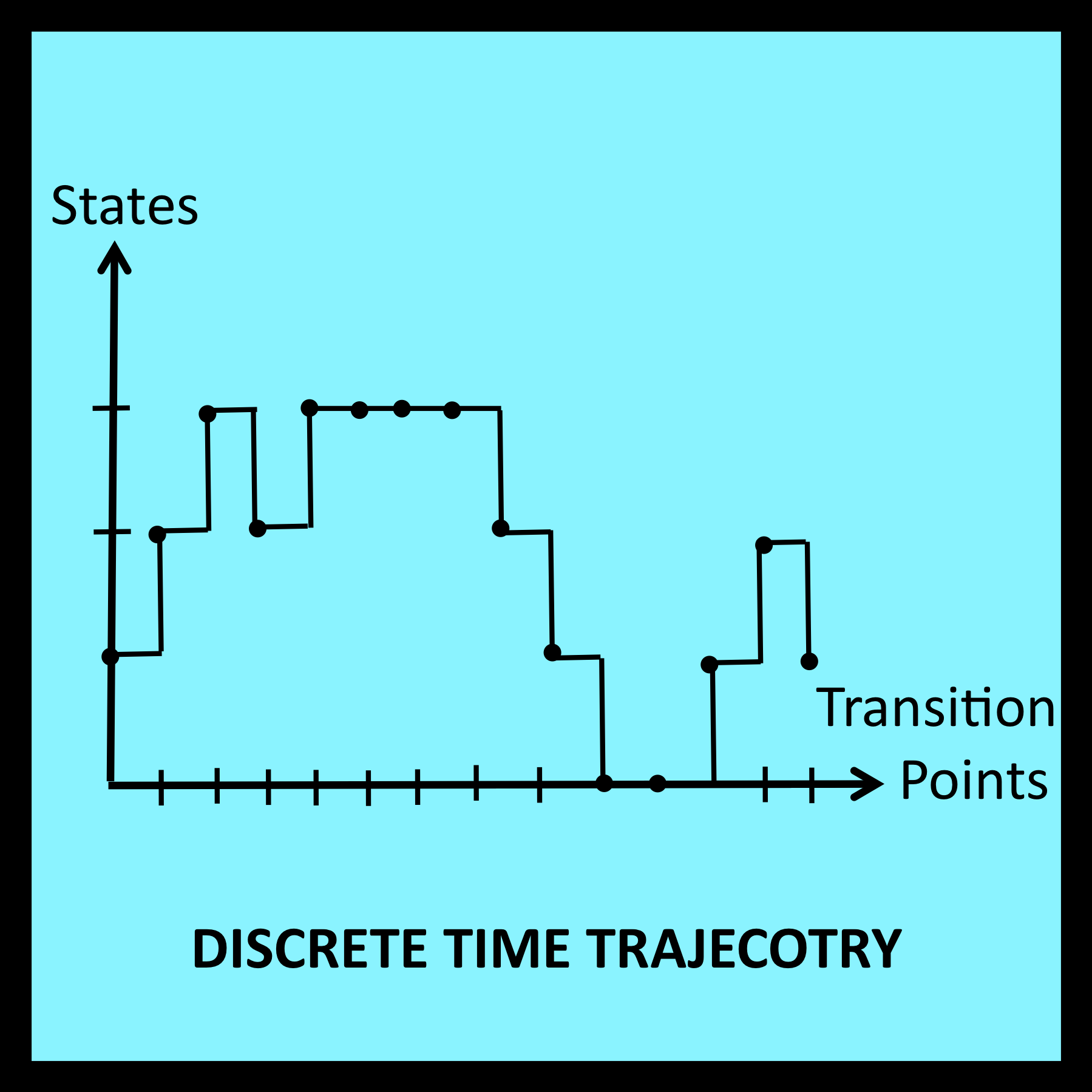The horizontal and vertical lines connecting the  dots in Figure 6-1 help the reader visualize the shape of the trajectory, but are not essential.  Similarly, the uniform spacing between each dot is also a visual aid.  It has no analytic significance because the elapsed time between each pair of successive transition points is unknown and thus cannot play a role in the analysis.

If the time of each transition is also available, the discrete time trajectory in Figure 6-1 can be transformed into a continuous time trajectory of the type illustrated in Figure 6-2.  In this case, the spacing between successive transition points is significant: it represents elapsed time.  This additional information can be applied to the analysis of the trajectory in Figure 6-2, making it possible to determine the proportion of time the walker actually spends at each station or in each state.  Expressions for the proportion of visits the walker makes to each station can also be derived, but are seldom the primary objective of the analysis.

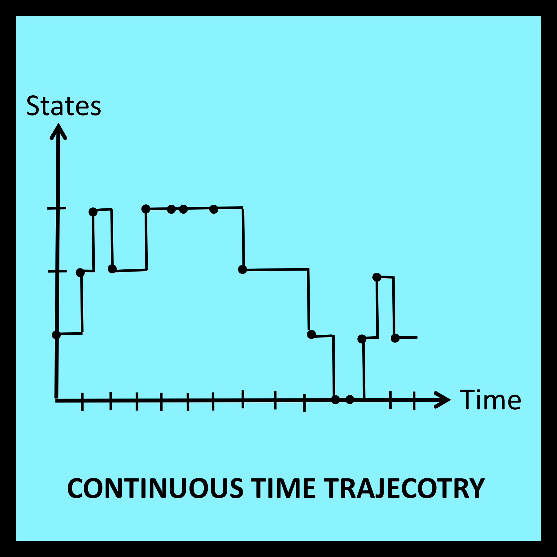One other difference between discrete time and continuous time trajectories concerns the amount of time spent in the final state.  In discrete time models, the last input symbol in a workload generates a transition into the final state of the trajectory.  This marks the end of the trajectory as indicated in Figure 6-1.    On the other hand, it is possible for a continuous time model to remain in the final state for an additional amount of time before the trajectory finally terminates.  Such a case is illustrated in Figure 6-2.

To accommodate this consideration, all workloads associated with continuous time LCD models must end with a special termination symbol: X.  The timestamp attached to the termination symbol X represents the instant at which the trajectory actually ends, and must be greater than or equal to the timestamp of the final state in the trajectory    Tables 6-2 and  6-4 in Section 6.5 illustrate the use of the special termination symbol.

6.2 Buffer overflow in continuous time

The simple random walk discussed in Chapters 1 through 5 is closely related to a buffering process that operates in continuous time.   In examples of this type, the state of the system being modeled corresponds to the number of items in a buffer rather than the position of a walker. Right and left turns correspond to increases and decreases in the number of buffered items, and rebounding off the reflecting barrier to the right of the highest state corresponds to dropping (i.e., discarding) an item that arrives when the buffer is currently full.

The next few sections describe this model in greater detail. As in the case of the random walk, the procedures used to analyze this specific example can be generalized to deal with a broad class of modeling problems. A number of these generalizations are described in Chapter 7.

6.2.1   The buffer/queue overflow problem

When requests for service arrive in a manner that is bursty rather than uniform, buffers are often provided to store incoming requests until they can be processed. Note that buffer capacity is always finite. Thus, as just noted, it may be possible for requests to arrive at a time when the buffer is already full. Such requests are typically dropped with the expectation that they will be transmitted again at some point in the future.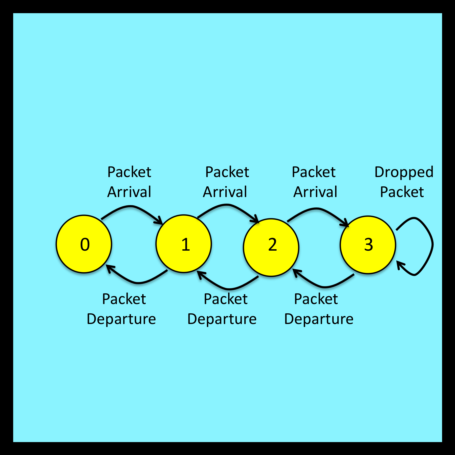

The designers of the ARPAnet, which is the predecessor of today’s Internet, anticipated this problem. They incorporated special algorithms into the software that implements the TCP/IP protocol to trigger such retransmissions automatically if a dropped packet is suspected. [Note: For purposes of this discussion, a packet is simply a short segment of a larger message. Packets are transmitted from router to router as they make their way across a network from their origin to their ultimate destination.]

Buffer overflow is no longer a concern for the powerful routers deployed in the backbone of the modern Internet. The processing capacity of these routers is matched to the maximum bandwidth of the lines that transmit incoming packets. As a result, these routers are able to complete the processing of a packet before the final byte of the next incoming packet (on that same line) arrives. This processing takes place in parallel for each line the router supports.

Buffer overflow can still be an issue for less advanced routers. It can also bring down web servers during periods of very high load (e.g., during denial of service attacks). The next few sections examine the buffer overflow problem for the simple case of a primitive router operating in a classical store and forward network.

.6.2.2 An LCD model of buffer operation

Note that buffer operation can be represented by the state transition diagram illustrated in Figure 6-3.   The number of packets in the buffer at any given instant corresponds to the state of the model. To simplify this particular example, the size of the buffer is set to an unrealistically small value of three. Extending this analysis to buffers with larger capacities is entirely straightforward.