1.1 Mathematics, measurement and the physical world
Physical objects and processes have existed in one form or another since the birth of the universe.   They are real entities whose existence does not depend in any way on the mathematical models that characterize their properties and behavior.  In contrast, mathematical models are pure creations of the human mind.  They exist in an abstract realm where they can be defined and analyzed without referring to physical entities of any type.

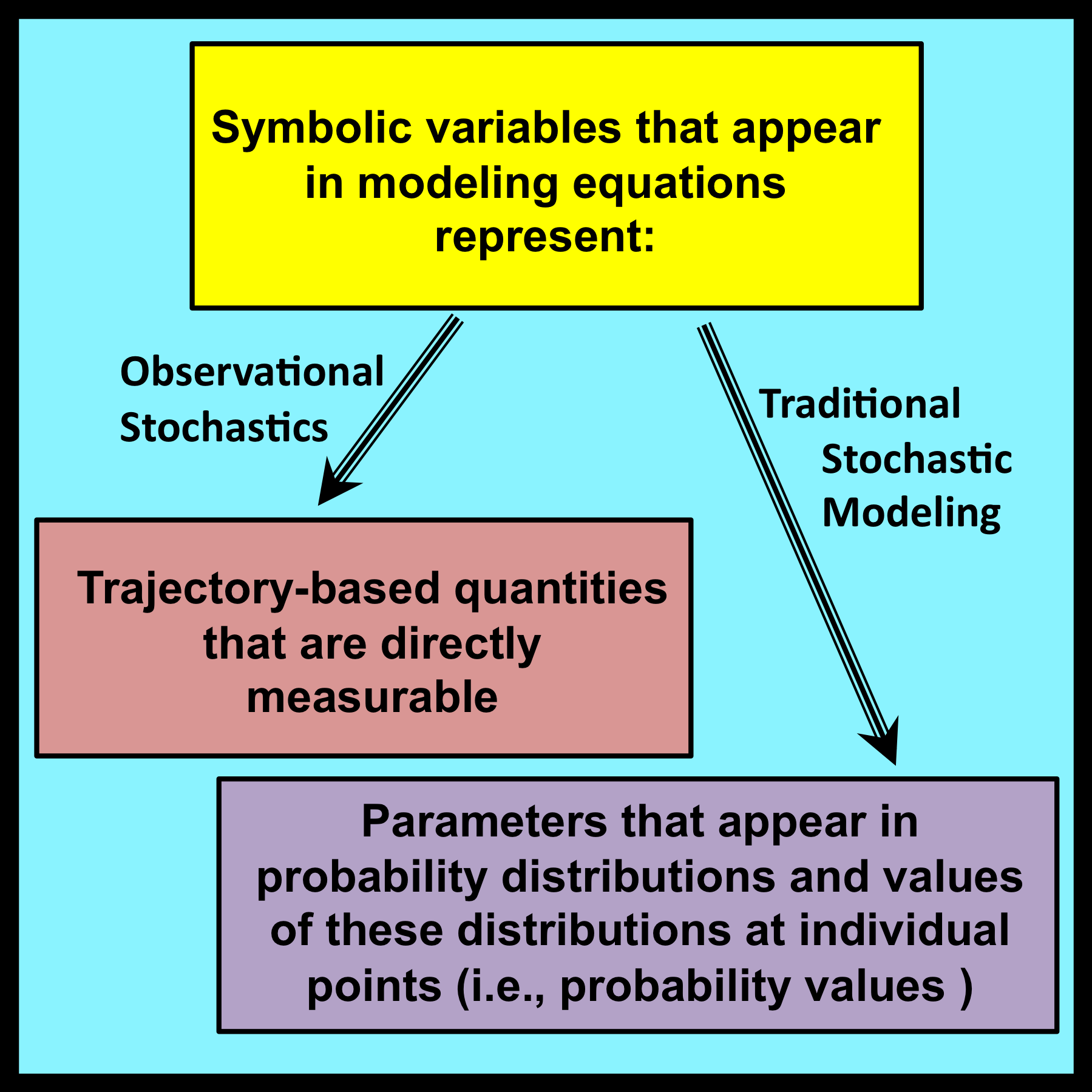
When mathematical models are applied to practical problems, the symbolic variables that appear in their associated equations are typically interpreted as measurable properties of corresponding physical entities.   In effect, the process of observing and measuring physical entities provides a crucial link that connects the realm of pure mathematics with physical reality. This linkage is immediately apparent in the work of engineers and experimental scientists who use mathematical models to solve problems that arise in the real world.

The connection between models and reality is not always so direct. One especially important exception arises when mathematical models are used to analyze processes whose detailed step-by-step behavior follows irregular patterns that appear to be the product of random factors.  In such cases, the observable properties of these processes are traditionally regarded as samples that have been drawn from underlying probability distributions.  The parameters that characterize these distributions (e.g., means, variances, etc.) appear as symbolic variables in the equations derived from such models.

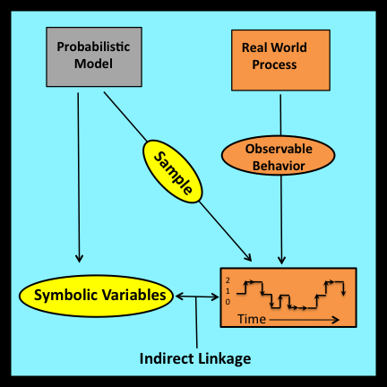Distributional parameters of this type differ fundamentally from the symbolic variables employed in conventional mathematical models. They are not linked directly to the observable properties of individual physical entities. At best, their exact values can be estimated with varying degrees of confidence to lie within ranges that are specified by sets of upper and lower bounds.

This book develops an alternative framework for analyzing systems and processes whose behavior appears to be driven by random (i.e., non-deterministic) forces. The new approach is based on a simple principle that is employed routinely in many other scientific disciplines: all symbolic variables that appear in the specification and solution of a mathematical  model must represent directly observable properties of the system or process being modeled. To highlight this point, the alternative framework will be referred to as observational stochastics.

In effect, observational stochastics complements traditional stochastic modeling by analyzing what are essentially the same physical phenomena from the perspective of individuals who apply mathematical models (i.e., practitioners) rather than theorists who work primarily in the realm of pure mathematics..  This alternative path leads to vastly simpler derivations of equations that are analogs of major results from stochastic theory, a different foundation for conceptualizing the intuitive notion of randomness and uncertainty (linked in spirit to nineteenth rather than twentieth century mathematics), new tests for determining whether or not a model’s assumptions are actually satisfied in practice, and new procedures for bounding errors when a model’s assumptions are not satisfied exactly.

1.2 Highlights of observational stochastics

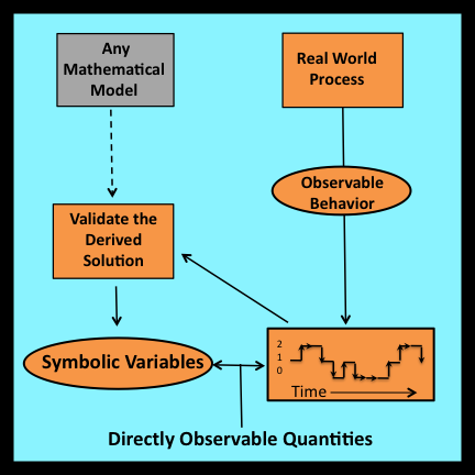Observational stochastics formalizes the procedures that practitioners follow when they validate mathematical models based on stationary (i.e., steady state) stochastic processes.  These validation procedures typically begin by observing the behavior of an actual system during a finite interval of time.  The objective is to determine whether or not the system’s behavior conforms to equations derived from the model being validated.

To make this determination, all symbolic variables that appear in these equations are associated with directly observable quantities.  These quantities are then measured so the equations can be evaluated numerically.  If the resulting computations generate predicted values that agree with their directly measured counter- parts, the validation is a success.

Observational stochastics employs several interrelated concepts to formalize the process of model validation. The next few sections provide brief descriptions of these concepts.  More detailed descriptions, along with numerous examples, are presented in the remaining sections of Chapter 1 and in the chapters that follow.

1.2.1 Interval-wide proportions

When analyzing a traditional stochastic model of a real or hypothetical system, one of the primary objectives is to derive the steady state probability distribution of the underlying stochastic process.  This distribution represents the chance that the system being modeled is in a given state at some instant of time.

While this characterization is meaningful within the realm of pure mathematics, the state of an actual system at any instant during a traditional validation experiment is not a distribution. It is instead a specific observable value.  This apparent mismatch is resolved by reinterpreting instantaneous probabilities as interval-wide proportions.  In other words, the steady state probability that the system is in some given state is equated to the proportion of time the system spends in that state during the entire validation interval.  The formal justification for this intuitively appealing assumption is based a subtle mathematical result, the Ergodic Theorem, which is discussed further in Section 2.7 and Section 9.2.

Observational stochastics avoids the reinterpretation issue entirely by dealing with observable interval-wide proportions from the onset. This shift in initial focus is one of the principal defining characteristics of observational stochastics.

1.2.2 Directly measurable variables

All symbolic variables employed in observational stochastics (including the interval-wide proportions mentioned in the preceding section) represent directly measurable quantities.  These variables are typically defined as ratios of raw counts and durations measured over entire intervals or over subsets of entire intervals.  Section 3.7 introduces a formal modeling  framework within which these directly observable variables can be defined.  Straight- forward procedures for measuring the values these variables attain in each specific instance are specified in Sections 3.7.3 and 3.7.4.

1.2.3 Directly verifiable assumptions

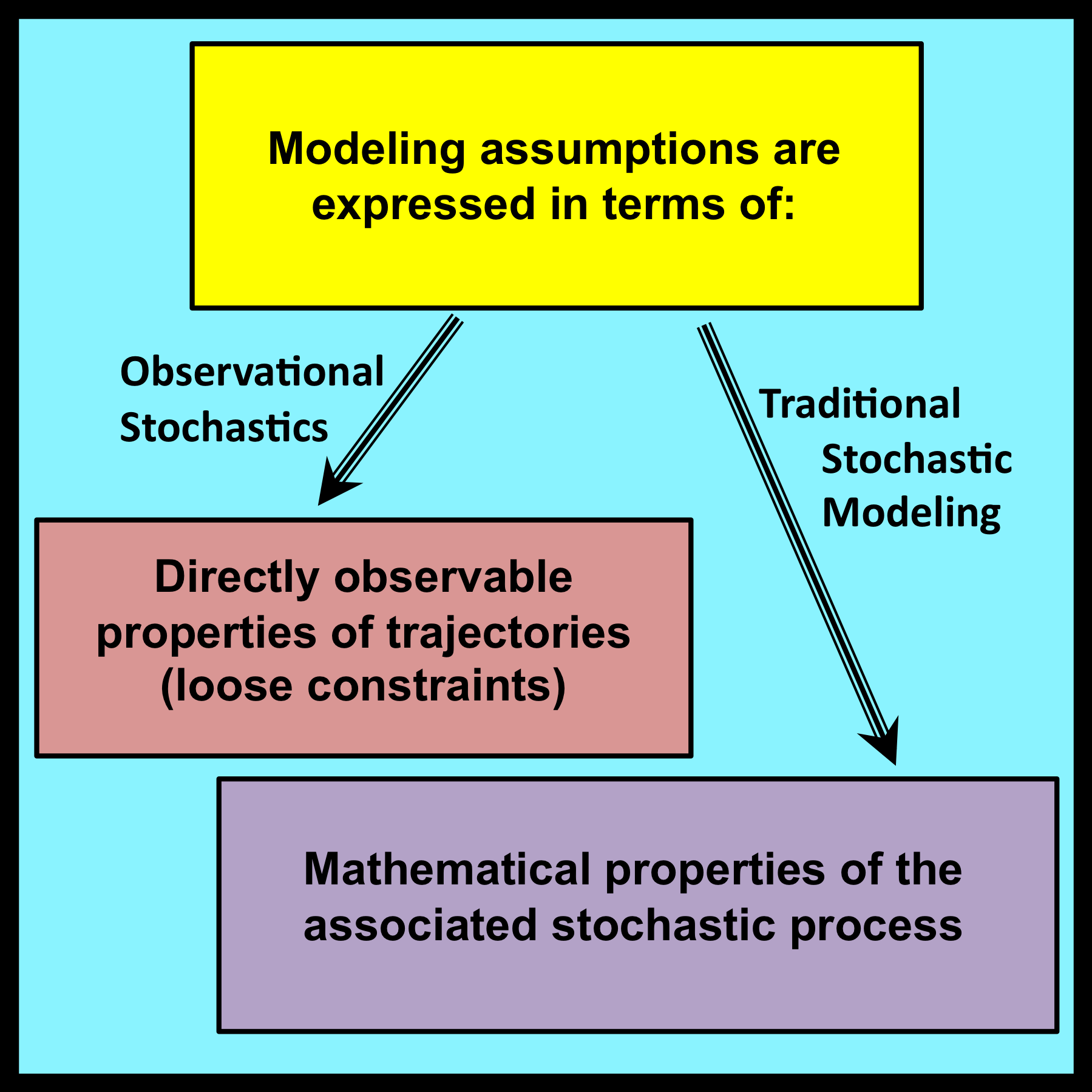
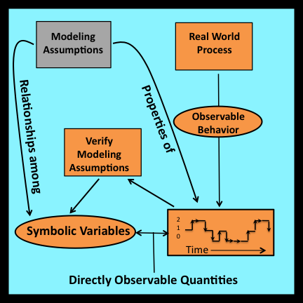
The assumptions employed in observational stochastics are expressed as algebraic relationships among symbolic variables that represent directly observable quantities.   To verify a particular assumption, the numerical values that these variables actually attain can be measured and then tested to determine if the corresponding algebraic relationship is satisfied.  If so, it is possible to conclude with complete certainty that the assumption is satisfied for the interval in question.

Verification procedures of this type are employed routinely in science and engineering.  However, because of the way randomness is represented in traditional probabilistic models, the assumptions incorporated into these models cannot be verified with complete certainty through straightforward procedures of this type.  The next section examines why this is so.

1.2.4 Sampling premise excluded

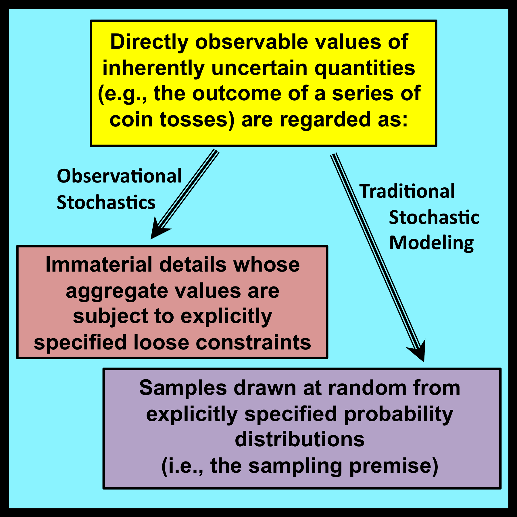
Mathematicians who deal with uncertainty typically associate the intuitive notion of randomness with the process of drawing samples from underlying probability distributions. The assumption that observed values can be regarded as samples drawn from such distributions will be referred to as the sampling premise.   In addition to its powerful intuitive appeal, the sampling premise provides the foundation for most – if not all –  traditional applications of probability and statistics.

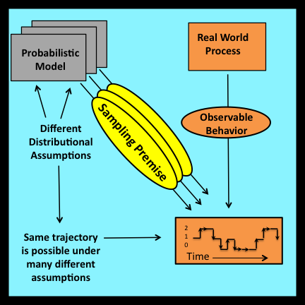Despite its nearly universal acceptance, the sampling premise does not represent a verifiable hypothesis. An unlimited number of different probability distributions can generate exactly the same set of observed values when a finite number of samples are drawn at random from these distributions.  Thus the validity of the sampling premise (for a given distributional form and a specific set of parameter values) can never be established with complete certainty by inspecting sets of observed values. Since observational stochastics requires directly verifiable assumptions, an alternative to the sampling premise must be introduced.

1.2.5 Loose constraints versus distributional assumptions

The primary role of the sampling premise is to provide a platform for specifying assumptions about the nature of the distributions incorporated into individual models. For example, the lengths of messages flowing through a communications network are often modeled as samples drawn from exponential distributions (Section 6.3).  Distributional assumptions of this type enable analysts to characterize the most important aspects of a process’s behavior, while allowing the step-by-step details to remain uncertain.

The new class of assumptions that are used within observational stochastics as replacements for the sampling premise are based on the simple idea of loose constraints.  Essentially, loose constraints are algebraic relationships among symbolic variables that represent directly observable quantities and serve as a model’s parameters (see Section 5.1.3).

The symbolic variables that appear in loose constraints correspond 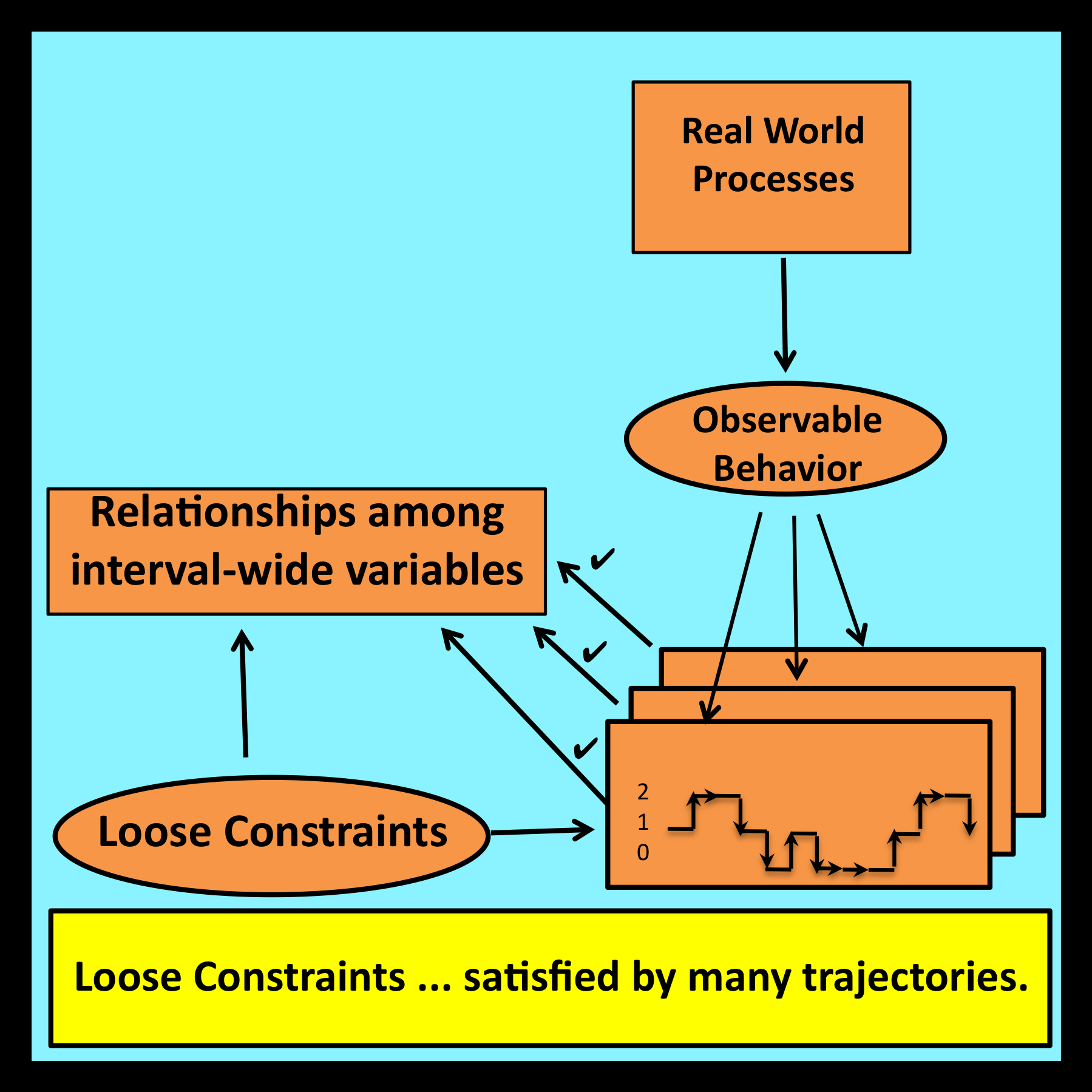to interval-wide proportions and averages. Individual observable values that are combined together to form these interval-wide quantities have no direct bearing on any results that are ultimately derived.  These individual observable values represent immaterial details whose exact values can, in principle, remain uncertain.

To illustrate the form loose constraints typically take, suppose a coin is tossed 1000 times.  Suppose further that 500 of these tosses actually come up heads.  Thus p, the observed proportion of heads, is equal to one half.

Now consider only those tosses that follow immediately after one of the 500 tosses that came up heads.   A typical loose constraint would require that the proportion of tosses that come up heads in this subset must also be equal to one half. More generally, a loose constraint might require that p, the overall proportion of heads observed for all tosses, must be equal to p-sub, the proportion of heads observed in some well defined subset of tosses.

Note that loose constraints of this type are directly verifiable.  They also allow immaterial step-by step details to remain uncertain.  There is no need to assume that the outcome of each coin toss corresponds to a sample drawn from a probability distribution. The sampling premise is never invoked.  In observational stochastics, it is sufficient to base an analysis entirely on relationships among directly observable quantities such as p and  p-sub.  In essence, observational stochastics replaces assumptions about the way observable values have been generated (i.e., the sampling premise) with assumptions about the way these values actually appear (i.e., assumptions expressed as loose constraints).

Many major results from the traditional theory of Markov processes, and from other branches of stochastic modeling, have direct counterparts that can be derived using such assumptions.  In addition to providing a simpler and more intuitive framework for their derivation, observational stochastics also demonstrates that these results are valid under conditions that are substantially more general than is commonly recognized.

Note that the mathematical relationships derived through observational stochastics apply to all trajectories that satisfy the loose constraints of the corresponding model.  This is analogous to the mathematical relationships derived through traditional stochastic models, which apply almost surely to the ensemble of sample paths associated with the underlying stochastic process.  These points are discussed further in Sections 6.9 and 9.2.

In contrast, the mathematical relationships derived using a conventional deterministic model apply only to a single trajectory whose detailed step-by-step structure is fully determined by the parameters of the deterministic model being analyzed. This distinguishes deterministic modeling from both observational stochastics and traditional stochastic analysis.

1.2.6 Loosely constrained deterministic (LCD) models

Validation experiments always involve two distinct entities: an abstract mathematical model and a physical system that can be observed and measured during an interval of time.   In traditional stochastic analyses, the abstract mathematical model is a stochastic process: that is, an ordered sequence of random variables indexed by integers or by real numbers.  The ordering represents the flow of time, and the probability distribution associated with each random variable in the sequence represents the distribution of states of the stochastic process at the corresponding instant.

Observational stochastics is based on a significantly different mathematical abstraction referred to as a loosely constrained deterministic (LCD) model (Buzen 2012).  LCD models reflect the fact that system behavior is typically controlled by a combination of deterministic and uncertain factors.  For example, when a new customer arrives at a queue, the length of the queue increases by one.  This increase is entirely deterministic.  However, the elapsed time between successive arrivals at a queue is typically uncertain.

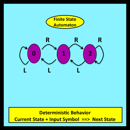
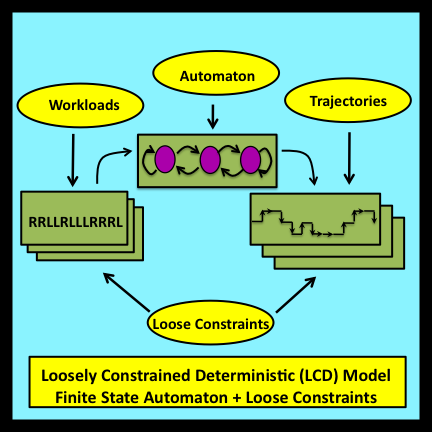Deterministic aspects of system behavior are represented within LCD models by formalisms adapted from Computer Science and  Electrical Engineering: specifically, finite state automata (Mealy 1955).  Loose constraints on the workloads processed by these automata and on the trajectories these workloads generate enable detailed aspects of system behavior to remain uncertain.

LCD models play a crucial role in observational stochastics by providing a rigorous foundation for the definitions of observability, measurability and system state.   Section 3.7 develops a formal characterization of LCD models and related concepts.

*

*

*

Table 1-1 summarizes the principal characteristics of observational stochastics and contrasts them with their traditional stochastic counterparts.  [The figures below illustrate the major points that appear in this table.]