5.1 Construction and application of LCD models

Chapter 3 introduced the notion of LCD models through a simple example: a random walk in one dimension with reflecting barriers.  This chapter presents a series of examples that involve the application of LCD models to systems whose behavior is somewhat more complex.  The modeling techniques described here are quite general and extend well beyond these specific examples.

Explicit algebraic solutions are derived in most cases, but these are of secondary importance.  The primary goal is to demonstrate how the basic building blocks that are available in observational stochastics can be used to solve a variety of problems.

5.1.1 Specifying the states of a model

The first step in the construction of any LCD model is to identify the set of states upon which the model will be based. For the random walks described in Chapter 3, state specification is both simple and intuitive: each station visited during a walk is represented by a separate state.  Thus, there is a direct one-to-one relationship between states and physical locations.

State specification is not always so straightforward. Sections 5.2 through 5.6 of this chapter illustrate the way states can be used to represent logical rather than physical entities. These examples deal primarily with behavior that is driven by the number of successive visits the walker makes to the same location.

Section 5.7 presents an entirely different example that illustrates the distinction between good and poor choices in the specification of a model’s states.  In this example, states correspond directly to simple physical entities and locations.  Nevertheless,  a substantial degree of insight and creativity is still required to select the most efficient set of states for a model that is developed to solve an intriguing mathematical puzzle.

Note that the state specification process is essentially the same for both LCD models and traditional stochastic models.  All the LCD models presented in this book have traditional stochastic counterparts that are based on identical sets of states.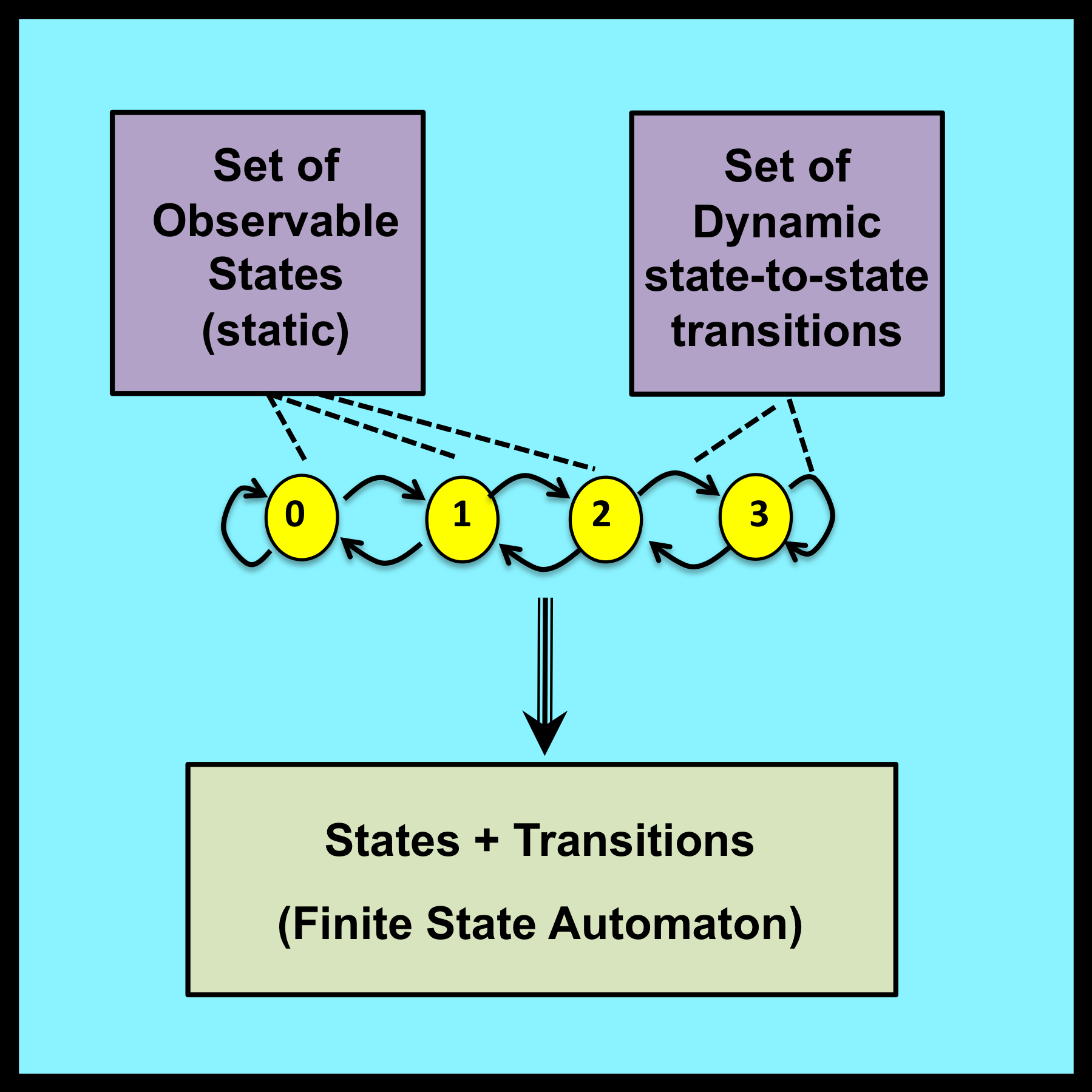

5.1.2 Specifying the dynamic behavior of a model

Once a set of states has been identified, the next step in the development of an LCD model is to specify the dynamic behavior of the system being analyzed.  In observational stochastics, the state of a system at any instant is a directly observable quantity. As a result, dynamic behavior can be characterized by trajectories that reflect the step-by-step changes in a system’s observable state that take place over an interval of  time.

Trajectories of this type can be specified by state transition diagrams or by finite state automata. For example, the state transition diagram shown in Figure 3-1 specifies the dynamic behavior of the simple random walk in Chapter 3.  The finite state automaton specified by equations (3-44) through (3-51) provides an alternative format for specifying the same information.

In a traditional stochastic model, the state of a system at any instant is characterized by a probability distribution.  As a result,  a system’s dynamic behavior can be specified by a sequence of probability distributions defined over an interval of time.  For the traditional random walk in Chapter 2, step-by-step variations in these probability distributions are specified by equations (2-9) through (2-12).  Equations of this type are used to characterize the dynamic behavior of all discrete time Markov processes.

5.1.3 Specifying the parameters of a model

Equations (3-44) through (3-51) and equations (2-9) through (2-12) are both used to specify dynamic behavior.  However, these two sets of equations differ in one fundamentally important respect. The first set of equations is “parameter free” while the second incorporates the distributional parameter r as well as the implicit distributional assumption of independent Bernoulli trials (which determines the joint distribution of the random variables that characterize the sequence of turns the walker makes).

In contrast, equations (3-44) to (3-51) are expressed solely in terms of input symbols (Ýand ß) and states (0, 1, 2 and 3).  There are no numerical parameters and no implicit assumptions.

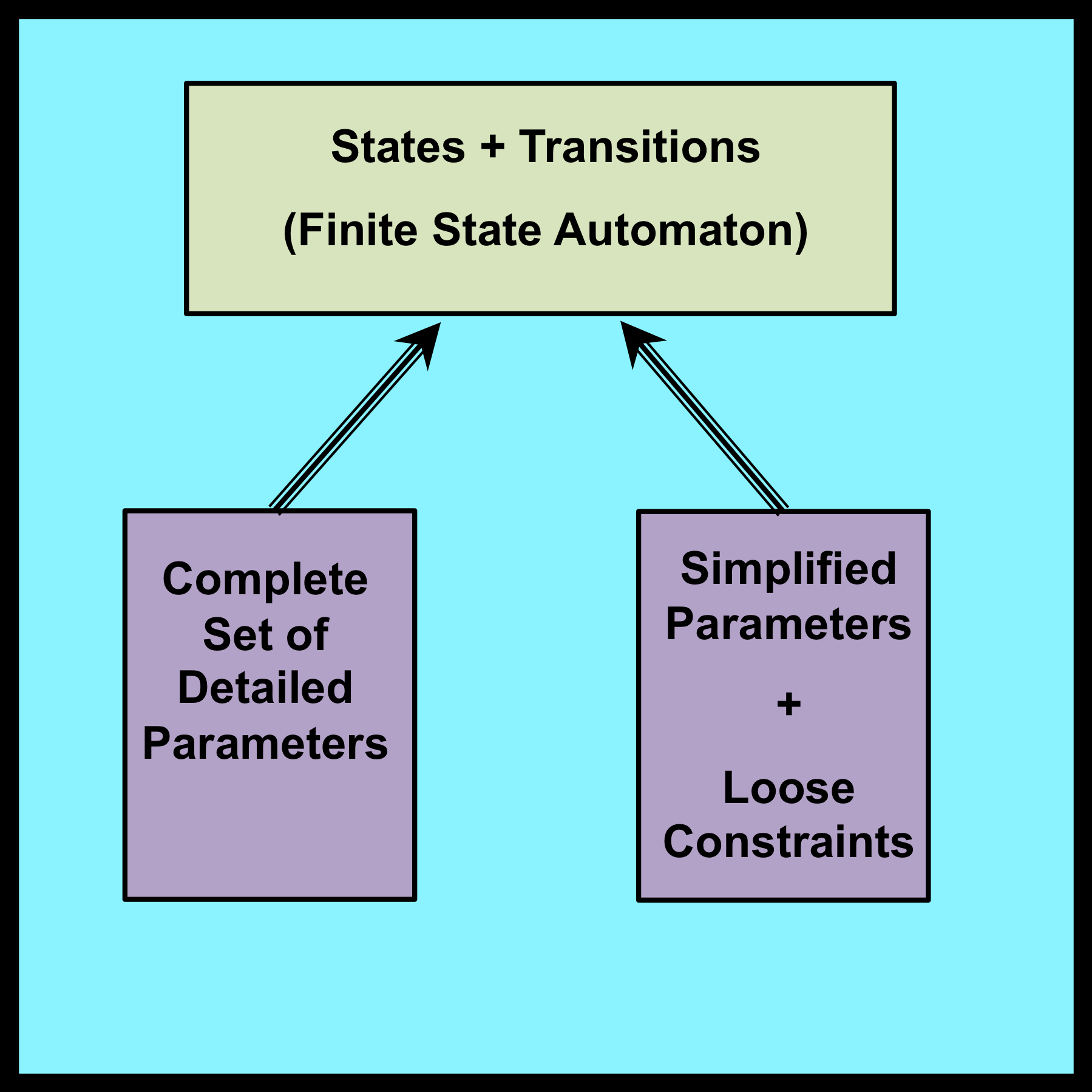
Since dynamic behavior is specified in a parameter free manner, the next step in the construction of an LCD model is to specify an appropriate set of parameters and modeling assumptions for the system being analyzed.  One option is to employ no modeling assumptions at all (except for the technical assumption of matched endpoints). This leads to a set of maximally detailed parameters.  For the simple random walk in Chapter 3, this maximally detailed set is: R(0), R(1), R(2) and R(3).  Results such as equations (3-30) through (3-33) that are expressed in terms of these maximally detailed parameters are, in general, applicable to all trajectories that can be generated by the model’s state transition diagram.

Solutions expressed in terms of maximally detailed parameters are of limited practical value because it is often unrealistic to assume that these detailed quantities can be estimated or predicted with an acceptable degree of accuracy.   To address this legitimate concern, LCD models provide a mechanism for reducing the total number of required parameters.  This reduction is achieved by introducing additional modeling assumptions that are expressed in terms of loose constraints.

Essentially, loose constraints are assumptions about relationships among the maximally detailed parameters of the original LCD model.  For example, the assumption that each turn a walker makes is empirically independent of the walker’s current location implies that all values of R(n) must be equal to a common value R.  Solutions derived under this assumption depend only on the value of R and are valid for all trajectories that satisfy this particular loose constraint.  The individual values of R(n) are immaterial.

The use of loose constraints to reduce the number of independent parameters in LCD models has no direct counterpart in traditional stochastic modeling.   However, this process plays a crucially important role in observational stochastics.

Note that loose constraints must also be intuitively plausible.  In other words, practitioners must have good reason to believe that the loose constraints incorporated into an LCD model are likely to be satisfied by trajectories that will be encountered during “what if” experiments that have not yet been conducted.  This issue is discussed further in Sections 6.4 through 6.8.  See especially the discussion of modeling risk in Section 6.7.1.

*

*

*

5.7 Structuring a model: the umbrella problem

The examples in Sections 5.2 through 5.6 are all variations of the same basic technique, which consists of adding special states to a model so that additional details can be represented. This section deals with a different modeling skill: identifying the most appropriate set of states to use when structuring a model.

The material in this section is adapted from an example described by Bertsekas and Tsitsiklis (2002, p. 329).   The example involves a professor who walks from home to school each day over the course of a semester.

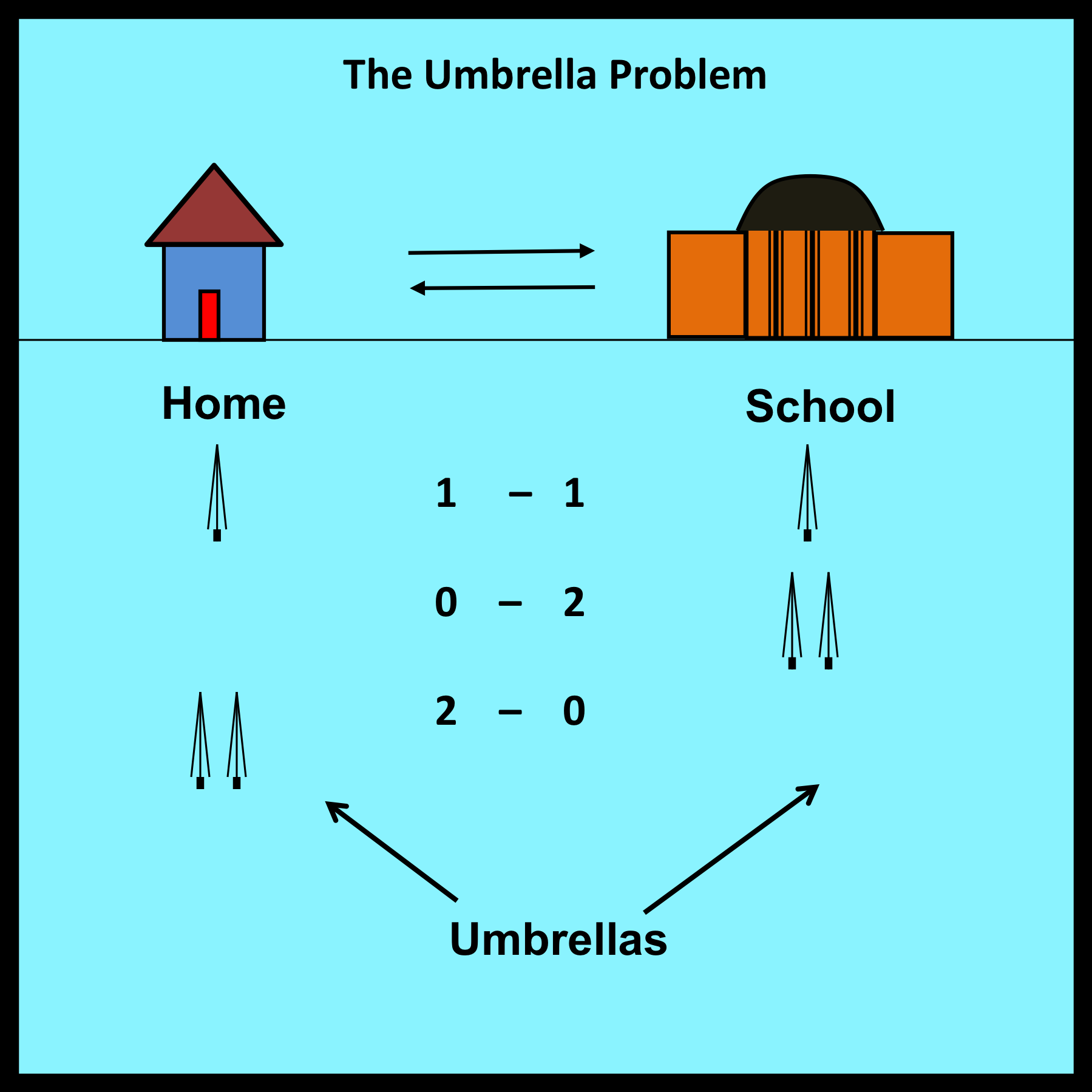The professor is concerned about getting wet during his daily commute, so he begins the semester by placing one umbrella at his home and one in his office. This guarantees that the professor will always have an umbrella available on the first rainy day. However, the professor is absent minded and never remembers to bring an umbrella back to its original location on sunny days. Thus, the professor may get wet on subsequent trips if he happens to be caught with no umbrella on a rainy day.

Assume that R represents the proportion of trips that begin while it is raining. The problem is to express W, the proportion of times the professor actually gets wet, as a function of R. To simplify the analysis, assume that it never begins to rain midway through a trip.

The fact that the professor travels back and forth between home and school is reminiscent of the random walks considered previously. However, the proportion of visits that the professor makes to each physical location is not the main issue here. Instead, the primary objective of the umbrella problem is to determine the fraction of trips that begin when it is raining and no umbrellas are available. The purpose of building a model is to evaluate the proportion of trips that begin under these circumstances.

To construct any model, it is necessary to begin by identifying a set of states and their associated transitions. In the case of the umbrella problem, two different models can be formulated: the first is straightforward, but somewhat cumbersome and overly complex. The second, described in Bertsekas and Tsitsiklis (2002), is elegant and insightful.

[Note: A standalone discussion of the Umbrella Problem and its solution appears in “The Observability Principle: Implications for Stochastic Modeling” – which can be downloaded from the Supplementary Material section of this website.]