 3.1 Characterization of observability
As discussed in Chapter 1, the variables used in observational stochastics represent quantities that are directly observable. This simple concept is easy to understand on an intuitive level. However, characterizing observability in terms that are both precise and broadly applicable is a challenging task. This is one of the main objectives of Chapter 3.
The analysis in the first part of this chapter deals with the simple random walk discussed in Chapters 1 and 2. A definition of observability within this context is developed in Section 3.2. This definition reflects the standard procedures that practitioners routinely employ when measuring actual systems. Sections 3.3 through 3.6 build upon this definition by presenting a formal analysis of random walks based entirely on the principles of observational stochastics.
Simple random walks also serve as a springboard for the general treatment of observability developed in Section 3.7. The discussion in Section 3.7 begins with the specification of an entity known as a loosely constrained deterministic (LCD) model. These LCD models (Buzen 2012) are used to develop a precise and broadly applicable characterization of observability. Observational stochastics rests upon the formal foundation that these models provide.
3.2 Observable variables for random walks 
The state transition diagram in Figure 2-1 can be regarded as representing the rules that govern a random walk. These rules specify the next station the walker will encounter after making a left or right turn. Note that the state transition diagram can also be used to infer information about the direction of each turn when only a trajectory such as the one shown in Figure 1-4 is available. For example, if station 2 is followed immediately by station 3 in a trajectory, the analyst can infer that the walker turned to the right after this particular departure from station 2.
The notion of turning to the right has meaning in the real world. On the other hand, the fact that station 2 is followed immediately by station 3 is a property of the trajectory itself. A trajectory for this random walk is simply a mathematical function that maps a sequence of integers – representing the step-by-step passage of time – into a set of states comprised of the integers 0 through 3.
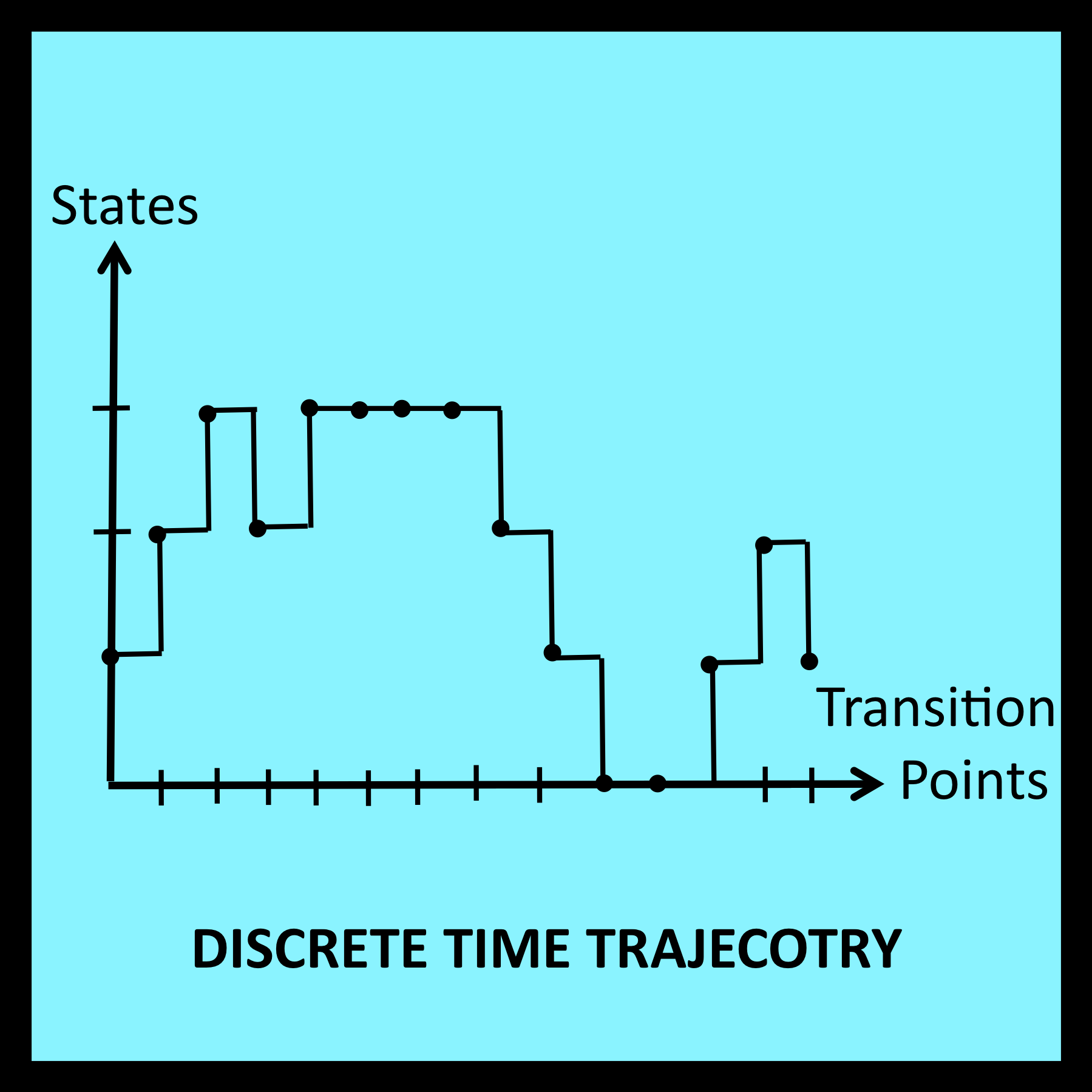
In this specific case, suppose an analyst is presented with a trajectory of the type shown in Figure 1-4. Assume the analyst knows that this trajectory was, in fact, generated by a random walk that conforms to the rules represented by the state transition diagram in Figure 2-1. It is then a routine matter for the analyst to extract the following values from the trajectory:
R(j)# = number of times the walker leaves station j and turns right
L(j)# = number of times the walker leaves station j and turns left
The hash tags incorporated into the symbols R(j)# and L(j)# highlight the fact that these variables represent basic measurements (i.e., raw counts) that can be regarded as directly observable properties of a trajectory.
Other observable quantities can now be expressed as simple functions of R(j)# and L(j)#.
*
*
*
*
3.7 Formal characterization of observational stochastics
As noted in Section 2.3, random variables and stochastic processes are abstract entities that exist within the realm of pure mathematics. To achieve a comparable level of rigor, the intuitive concepts employed in observational stochastics must also be defined in formal mathematical terms.
Practitioners who are comfortable with the intuitive notions of system, workload, trajectory and observable quantity, and who have a limited interest in mathematical formalisms, may wish to skip the material in the next few sections and proceed directly to Chapter 4.
3.7.1 State transition diagrams and finite state automata
On an intuitive level, state transition diagrams use simple graphical conventions to represent the step-by-step behavior of real or hypothetical systems. It is assumed that these systems can be in a number of different observable states. Each state is represented by a non-negative integer and is displayed within a circle as shown in Figure 2-1. The total number of states must be finite.
System behavior is driven by a sequence of external events. Some of these external events cause the system to enter a new state. Others leave the current state unchanged. Each such transition is represented by a transition arrow that connects the current state to the state the system enters immediately following the corresponding external event. If the current state and the next state are the same, the transition arrow loops back to the current state. Such loops are shown in Figure 3-1 at states 0 and 3.
Formally speaking, states are simply mathematical abstractions labeled with the integers 0 through N. Their interpretation is entirely arbitrary and consistent with Kolmogorov’s (1933) characterization of the states in a state space: “What the elements of this set represent is of no importance in the purely mathematical development of the theory.”
Transition arrows are ordered pairs of states (j, k) where state j is connected to the tail of the arrow and state k is connected to its head. Each transition arrow is associated with one or more input symbols. Input symbols are mathematical abstractions whose interpretations are once again entirely arbitrary. On an intuitive level, input symbols correspond to external events.
*
*
*
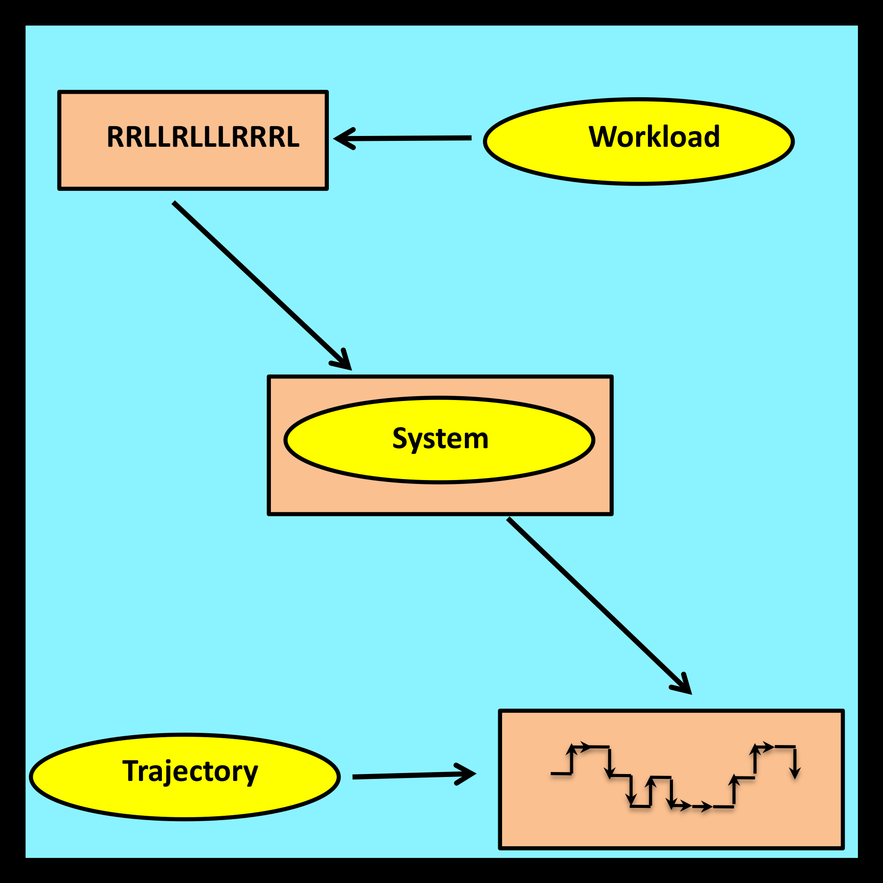
3.7.2 Workloads, trajectories and compound trajectories 
A workload is an ordered string of input symbols. In observational stochastics, the number of possible input symbols in a workload is always finite.
*
*
*
A trajectory is an ordered string of states: s(0), s(1), s(2) … . Intuitively, a trajectory is generated when a workload is processed by a finite state automaton.
[ A Loosely Constrained Deterministic (LCD) Model is a finite state automaton (finite state machine) together with a set of loose constraints on the workloads and trajectories associated with this automaton.]
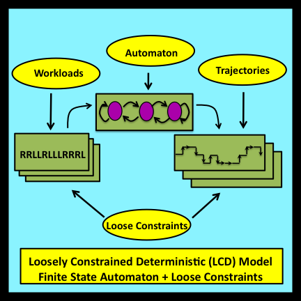
[… As in the case of a traditional stochastic model, the results derived through an LCD model apply to an entire set (ensemble) of associated trajectories: in this case, derived results are guaranteed to be valid for all trajectories that are consistent with the structure imposed by the model’s finite state automaton and also satisfy the model’s loose constraints. The step-by-step details of these trajectories are immaterial to the analysis and can remain uncertain. There is no need to assume that these observable details are the result of sampling from underlying probability distributions.]