4.1 Overview

The principles of observational stochastics extend well beyond the specific example presented in Chapter 3.  In fact, observational stochastics is applicable in many situations where Markov models would otherwise be employed.  This chapter builds upon the concepts and techniques presented earlier in order to develop these extensions.

Even though the overall flow of the analysis is quite similar to Chapter 3, the mathematical notation required to deal with the general case adds complexity to the discussion.  Readers interested in the applications of observational stochastics rather than the mathematical equations that must be solved when dealing with the general case may wish to review the following seven points and then proceed directly to Chapter 5.

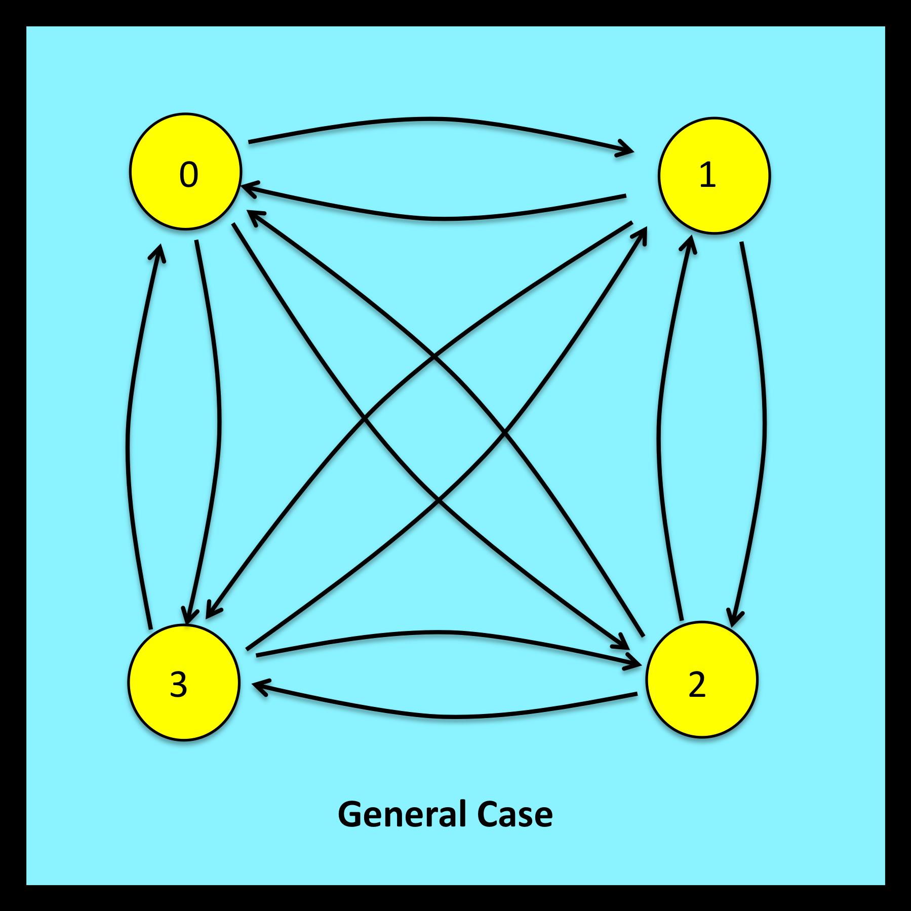
1. The techniques used in Chapter 3 to analyze the simple random walk can be extended to deal with random walks where the number of stations is equal to any value N and where each station can be reached from every other station in a single step.
2. In this very general setting, the objective once again is to determine the proportion of visits the walker makes to each station over the course of the trajectory. These observable proportions are represented symbolically as P(0), P(1), P(2) … P(N).
3. If the endpoints of a trajectory are matched, the desired values of P(j) are given by the solution to a set of balance equations obtained by setting the number of entrances into each station equal to the number of exits. These balance equations are direct generalizations of equations  (3-18) through (3-21).  The entire set of balance equations are specified  using standard mathematical notation in equation (4-22).
4. If the endpoints of a trajectory are not matched, the solution to the balance equations still provides a reasonable approximation to the actual values of P(j). This is true in most, but not all, cases. In the limit as trajectory length increases, the error associated with this approximation usually approaches zero.  When required, exact solutions for trajectories with unmatched endpoints can be obtained through the analysis presented in Section 4.7.2.
5. The form of the general algebraic solution – with or without matched endpoints – is algebraically complex and of limited interest. Practitioners are typically concerned with solutions to specific sets of balance equations that are associated with individual models such as those presented in Chapters 3 and 5.
6. Trajectories with matched endpoints are closely related to a new class of formal objects known as t-loops (trajectory loops). To construct a  t-loop,  simply merge the initial and final stations of a trajectory with matched endpoints.  This transforms the original  linear trajectory into a closed loop with no beginning and no end.  Some interesting properties of t-loops are noted in section 4.7.4.
7. The general solution for the values of P(0), P(1), P(2) … P(N) obtained using observational stochastics has exactly the same algebraic form as the steady state distribution of the corresponding Markov chain.   However, in a traditional time-homogeneous Markov chain, the transition probabilities that control step-by-step behavior are the same for every step of an associated trajectory.  In contrast, the global transition matrices employed in observational stochastics are comprised of overall values derived from complete trajectories.  The detailed step-by-step mechanisms that regulate these trajectories have no impact on the analysis and remain immaterial.   This enables derived results to apply more broadly. This issue is discussed in general terms in Section 4.8 and also revisited in Section 5.6 of Chapter 5.