2.1 Overall goals of this chapter

Chapter 1 introduced the concept of a simple random walk and  discussed several implications of equations (1-1) through (1-4).   However, these equations were not derived in a rigorously formal mathematical sense.  This chapter presents a derivation within the context of traditional stochastic analysis.  A number of basic concepts from the theory of probability and stochastic processes are reviewed in greater detail than is customary.  Readers already familiar with these aspects of stochastic modeling may wish to skip this chapter entirely and proceed to Chapter 3.

2.2 Deterministic state transition diagrams

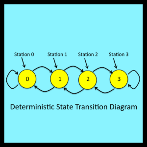
To begin the analysis, note that the transitions that take place during the random walk discussed in Chapter 1 can be represented by the state transition diagram shown in Figure 2-1. The circles in this figure represent the four stations, and the arrows represent the possible station-to-station transitions that can take place during a single step. Even though the walk is classified as random, the diagram in Figure 2-1 is clearly deterministic: if the walker is currently at station 1, and if the next turn is to the right, the walker will always move to station 2.

All the other transitions shown in Figure 2-1 are equally deterministic. Most “random” systems that are analyzed using stochastic models have a deterministic core that can be specified using a state transition diagram of the type illustrated in Figure 2-1.

2.3 The traditional characterization of uncertainty

The next issue to consider is the nature of the mechanism that causes the walker to move from station to station as the walk proceeds.   In order for the walk to be random, the sequence of left and right turns that directs the walker’s movements from station to station must be inherently uncertain.   One way to represent this type of uncertainty is to assume that the walker tosses a coin before leaving each station. If the coin comes up heads, the next turn is to the right; if it comes up tails, the next turn is to the left.

2.3.1 Sample spaces and probabilities

The abstract notion of sets and their members provides the standard mathematical foundation for dealing with uncertainty. Essentially, the members of a set are used to represent the possible outcomes of a process that is inherently uncertain. Such sets of possible outcomes are referred to as sample spaces.

In the case of a random walk, the set {heads, tails} is used to represent the possible outcomes of each coin toss.   There is, of course, a direct connection between the observable outcomes of an actual coin toss and the members of this sample space. However, the set {heads, tails} can also be regarded as an abstract entity whose existence is entirely independent of the physical world.   As such, its only properties are those defined within the formal domain of set theory: union, intersection, and so on.

The next step in the conventional representation of uncertainty is to associate a probability with each member and each subset within a sample space. A probability is simply a non-negative real number. The probability associated with an entire sample space must be equal to 1. Also, the probabilities that are assigned to subsets must satisfy the simple and entirely straightforward rules of measure theory: most importantly, if two subsets are disjoint, the probability assigned to their union must be equal to the sum of their individual probabilities.

Technically speaking, there is no need to specify a connection between probabilities and observable properties of processes that operate in the real world. This connection lies beyond the formal boundaries of the theory of probability. However, as discussed in Chapter 8, Bayesians and frequentists have clear but differing views regarding the connection between abstract mathematical probabilities and observable properties of processes that operate in the real world. These views are based on principles that have strong intuitive appeal, but neither view can be proven correct in any rigorous sense. Simply put, the theory of probability as formalized by Komogorov (1933) imposes no assumptions about the connection between probabilities and real world observables.

2.3.2 Random variables

A sample space, together with its probability distribution, is referred to as a random variable. Most of the results derived from probabilistic models are expressed in terms of random variables and their associated probability distributions.

For the random walk being discussed here, the outcome of each successive coin toss is represented by a separate random variable. For each of these random variables, the sample space is the set {heads, tails}, the probability associated with heads is equal to r, and the probability associated with tails is equal to 1-r. This sequence of identically distributed random variables, together with the relationships represented in Figure 2-1, provides the basis for a traditional stochastic model of a random walk.