7.1 Overview

The first few sections of this chapter extend the analysis in Chapter 6 to the general case where LCD models can include an arbitrary number of states and an arbitrarily connected state transition diagram.   The development of these extensions closely follows the approach employed in Chapter 4; however, in this chapter it is assumed that time advances continuously rather than in discrete steps.   

The main objective is to demonstrate that real world systems that are traditionally modeled as continuous time Markov processes can also be viewed through the lens of observational stochastics and modeled as continuous time LCD models.   Even though the underlying assumptions are markedly different, the attained distribution derived from the LCD model will have exactly the same algebraic form as the steady state distribution derived from the corresponding Markov model.  Thus, the two models yield exactly the same results for a large class of practical problems.

As in the case of Chapter 4, the mathematical notation required to deal with the general case adds complexity to the discussion.  Readers interested in the applications of the analysis rather than the mathematical details of the general solution, may wish to review the following points and then proceed directly to Section 7.7.  These seven points are direct analogs of their counterparts in Chapter 4.

1. The techniques used in Chapter 6 to analyze the buffer overflow problem can be extended to deal with continuous time LCD models where the number of states is equal to any value N and where each state can be reached from every other state in a single step.
2. In this very general setting, the objective is to determine the proportion of time spent in each state over the course of the trajectory. These observable proportions are represented symbolically as p(0), p(1), p(2) … p(N).
3. If the endpoints of a trajectory are matched, the desired values of p(j) are given by the solution to a set of balance equations obtained, as usual, by setting the number of transitions into a state equal to the number of transitions out. These balance equations, which are specified in Theorem 7.1, are direct generalizations of equations (6-19) through (6-22).
4. If the endpoints of a trajectory are not matched, the solution to the balance equations still provides – in most cases – a reasonable approximation to the actual values of p(j). In the limit as trajectory length increases, the error associated with this approximation usually approaches zero. If necessary, exact solutions for finite length trajectories with unmatched endpoints can be obtained through the procedure specified in Corollary 7.1.
5. The form of the general solution – with or without matched endpoints – is mathematically complex and of limited interest. Practitioners are typically concerned with solutions to balance equations that are associated with specific models such as the buffer overflow model in Chapter 6 and the various queuing models that will be discussed later in Chapter 7.
6. The t-loops introduced in Section 4.7.4 can be extended to represent continuous time processes. These extensions create richer structures with additional mathematical properties.
7. The general solution for the values of p(0), p(1), p(2), … p(N) obtained using observational stochastics has exactly the same algebraic form as the steady state distribution of the corresponding continuous time Markov process. However, the transition rate matrix that defines a traditional continuous time Markov process is comprised of instantaneous transition rates that must remain stationary (i.e., time-homogeneous) throughout the entire trajectory. In contrast, the global transition rate matrices employed in observational stochastics are comprised of average rates for entire trajectories. The detailed instant-by-instant forces that shape these trajectories have no impact on the analysis and need not be stationary.   This again enables observational results to apply more broadly than the corresponding stochastic results.

*
*
*

7.11 Selected examples of practical significance

Queuing theory can be applied to many problems that arise during the design, analysis and day-to-day management of modern computer systems and communication networks. The examples in the last few sections have barely scratched the surface of this important subject. This section presents brief descriptions of three queuing models whose impact remains substantial more than four decades after their original development.

Solutions to the models discussed in this section are algebraically complex. This makes it difficult to derive useful intuitive insights by direct inspection of the solutions themselves. Nevertheless, it is important for practitioners to understand the assumptions that lie behind the corresponding models and the limitations that these assumptions impose.

7.11.1 Open queuing networks: ARPAnet and Internet

In certain situations, the output of one queue is linked to the input of another. Multiple queues connected in this manner form a queuing network as shown in Figure 7-13. Models of this particular type are referred to as open networks because customers are free to enter and leave: thus the number of customers actually in the network fluctuates over time.

Len Kleinrock (1962) pioneered the application of such models to the analysis of store and forward computer networks. His work has had a major impact on the modern world. Today’s Internet is a direct descendant of the ARPAnet, a computer network developed in the late 1960s under sponsorship of the Department of Defense Advanced Research Projects Agency (ARPA).

During the earliest phases of this project, Kleinrock’s models were used to determine whether or not such a network would ever be able to deliver satisfactory levels of performance. The decision to move ahead with funding for the project depended on the results of Kleinrock’s analysis, which was carried out before a single line of code was written (Severance 2014). Later, Kleinrock’s lab at UCLA hosted the first node on the ARPAnet and was the point of origin for the first packets actually transmitted over this network.

The analysis in Kleinrock’s PhD dissertation includes a highly detailed queuing model that keeps track of the properties of individual messages as they move from node to node. Representing message flow at this level of detail leads to a model of enormous mathematical complexity. To obtain a closed form analytic solution, Kleinrock introduced a profoundly important simplifying assumption. In essence, this assumption enabled each node to be separated from the rest of the network and modeled as an independent queuing server.

As part of his PhD dissertation, Kleinrock also constructed a detailed simulation model that actually tracked the identities of individual messages. When he compared the results of his detailed simulation with the approximate analytic model, he discovered that the differences were relatively small and that the additional details incorporated into the simulation model did not have a material effect on the main results of his analysis. From the perspective of observational stochastics, Kleinrock’s simplifying assumption has much in common with the assumption that online behavior is equal to off-line behavior: both lead to acceptably accurate queuing models even though certain details are not represented precisely.

7.11.2 Closed queuing networks: computer performance

Figures 7-2 and 7-6 are examples of closed queuing networks. A fixed number of tokens (customers) circulate around these networks at all times. There are no infinite source servers capable of injecting new customers into the network; conversely, customers who are in the network at time zero have no way to exit.

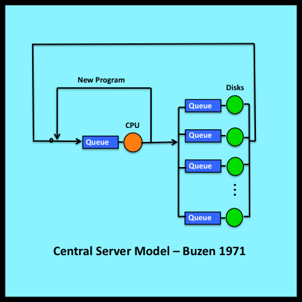
Figure 7-14 illustrates an especially useful closed queuing network known as the central server model (Buzen 1971, 1973). This model represents a multiprogrammed computer system operating under a steady backlog. Each token circulating around this network represents an active program. Program behavior is characterized as an alternating sequence of CPU processing bursts and I/O transfers. When a program terminates, its associated token moves along the “new program” loop and returns representing the first processing burst of the next program waiting in the backlog. Thus the rate at which tokens flow through the new program loop represents the throughput of the system being modeled.

The central server model is well suited for analyzing the benefits of increasing memory size, upgrading processor speed or the number of tightly coupled processors (SMPs), and upgrading I/O device performance by installing faster devices, cached storage controllers, or solid state disks. The model is particularly useful for identifying bottlenecks and for assessing alternative strategies for alleviating these bottlenecks.

A generalized closed form solution for queuing models of this type was originally derived by Jackson (1963) and, independently, by Gordon and Newell (1967). The solution constitutes a major milestone in queuing theory. However, for a closed model with N circulating customers and M servers, the number of possible states is equal to M+N-1factorial divided by the product of N factorial and M-1 factorial: that is, (M+N-1)!/[N!(M-1)!]. This number grows explosively as M and N increase, making direct evaluation of the closed form solutions derived by Jackson and by Gordon and Newell computationally intractable for all but the simplest of models. As a result, these solutions attracted little attention from researchers and practitioners for several years.

The situation changed abruptly in the summer of 1970 with the discovery of a powerful set of recursive relationships among the elements of the closed form solutions. These relationships provided the basis for remarkably efficient iterative algorithms for evaluating Gordon and Newell’s general solution (Buzen 1971, 1973). These same recursions also yielded simple algebraic expressions for related quantities that are difficult to evaluate directly: for example, the marginal queue length distribution for each server in a queuing network (which can then be used to compute mean queue lengths, percentiles, etc.). See Bruell and Balbo (1980, pp. 36-55), Harrison and Patel (1993, pp. 235-238), Bolch, Greiner, de Meer and Trivedi (2006, pp. 369-384), Stewart (2009, pp. 570-581), or Gelenbe and Mitrani (2010, pp 106-114) for extended discussions of this approach, now known as the convolution algorithm or Buzen’s algorithm (Wikipedia).

In combination with Jackson’s general solution, the central server model and the availability of efficient computational algorithms ignited a surge of activity by an international community of researchers. This led to a rapid succession of major advances in the theory of queuing networks and to the development of other efficient computational algorithms for the evaluation of these networks.

These advances, which are described in the texts cited in the preceding paragraph and in other texts cited in the Preface, were soon incorporated into commercially successful modeling tools (Buzen, Goldberg, Langer, Lentz, Schwenk, Sheetz and Shum 1978). Tools of this type have been used for decades to manage performance and plan capacity at many of the world’s largest data centers (Casale, Gribaudo and Serazzi 2010). Queuing network models remain important tools in the modern era of cloud computing, service oriented architecture, resource virtualization and big data.

7.11.3 The ALOHA network: origins of Ethernet

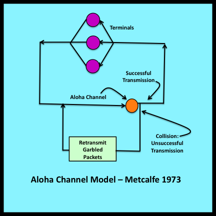
The ALOHA system was an early computer network designed by Norm Abramson of the University of Hawaii (Abramson 1970). In this network, user terminals on separate islands communicated with a centrally located computer system via a radio link. All terminals shared a single UHF channel for sending inbound packets. A second channel was used at the central site for outbound responses.

One of the most challenging problems in this environment is managing access to the shared channel used for inbound packets. Since the terminals are geographically remote, there is no easy way to coordinate this access. Abramson’s solution is noteworthy for its simplicity and its audacity: the basic idea is to allow each terminal to operate with complete disregard for what other terminals may or may not be doing. In this chaotic environment, some packets get through; others are garbled because they are sent at times when the channel is already busy. To accommodate such failures, the central system sends back an explicit acknowledgement when an undamaged packet is received. If a terminal does not receive an acknowledgement within a specified timeout window, the terminal assumes that a collision has occurred and retransmits the packet.

Abramson constructed a queuing model to determine the maximum effective utilization of a basic ALOHA channel. [Effective utilization is utilization due to newly arriving packets. It does not include the load generated by retransmitted packets.] Abramson showed that the maximum effective utilization of a basic ALOHA channel is equal to 1/2e (approximately 18%), where e is the mathematical constant 2.718… .

Abramson’s model incorporates an infinite source arrival process of the type depicted in Figure 7-3. Each terminal in Abramson’s model generates an independent stream of new packets. All terminals generate packets at the same basic rate. Thus, if there are N terminals, the total arrival rate for new packets is N times this basic rate. An assumption of this type is not uncommon and can be found in many queuing models.

Bob Metcalfe recognized that this assumption has certain undesirable implications when applied to the analysis of “what if” questions that involve increasing the number of terminals. Imagine a case where terminals are added (one by one) to an ALOHA network. As long as effective utilization remains below 1/2e, the network will be stable and Abramson’s model will yield a well defined result. However, at some point adding the next additional terminal will cause the total effective utilization to exceed 1/2e. At this point, the model predicts that the channel will become unstable due to an “uncontrolled regenerative burst of retransmission.” (Metcalfe 1973, Chapter 5)

Based on his practical experience with networks, Metcalfe regarded such a catastrophic collapse (triggered by the addition of a single terminal) as unlikely and unrealistic. He believed that ALOHA networks will remain stable as each new terminal is added and that the number of terminals in retransmission mode – and thus the total number of retransmissions per second – will increase gradually (rather than abruptly) during this process.

Metcalfe went on to develop a queuing model that predicts this type of behavior for his PhD dissertation. (Metcalfe 1973) In his revised ALOHA model, the load on the network is generated by a finite source arrival process of the type depicted in Figure 7-6. Abramson’s limit of 1/2e for effective utilization is still applicable, but this limit is now approached in a smooth asymptotic fashion as the number of attached terminals increases.

During the course of his analysis, Metcalfe recognized that the performance of ALOHA-like networks could be improved substantially by testing the status of the channel immediately prior to sending a packet, and by only transmitting packets when the channel is free. This testing procedure is known as carrier sensing. It reduces, but does not completely eliminate, the proportion of packets that collide with one another and have to be retransmitted. Collisions can still occur if two terminals detect a “not busy” condition at the same time and then decide to initiate transmissions concurrently.

Metcalfe’s research on ALOHA led to another important insight: he recognized that ALOHA-like networks augmented with carrier sensing would be especially useful in settings where terminals are relatively close geographically and are connected by physical wires rather than a radio channel. The Ethernet protocol, which is the de facto standard for most of today’s local area networks, began as a practical application of this insight.

Bob Metcalfe successfully defended his PhD dissertation with its refined model of the ALOHA network in May 1973. The following week he returned to California and coined the term Ethernet in an internal memo written at Xerox PARC (Palo Alto Research Center). Metcalfe and his colleague David Boggs had the first Ethernet LAN up and running at PARC six months later.

There is, of course, much more to this story (Metcalfe and Shustek 2006), but it remains a compelling example of the link between queuing models and inventions that have had a profound impact on the modern world.