Why read this book?
Students will better understand how their classroom/textbook material is actually applied in practice.
Practitioners (including engineers and experimental scientists) will discover new ways to explain and justify their modeling results to non-specialists … and new ways to assess the level of risk inherent in these results.
Theoreticians and advanced students will find opportunities to explore and extend the new mathematical structures that are introduced in this volume.
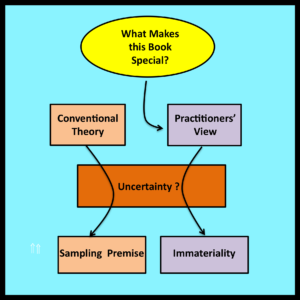
What makes this book special?
Rethinking Randomness is written from the perspective of practitioners who apply stochastic models to the analysis of real world systems. This is important because practitioners and theoreticians deal differently with the issues of observability and uncertainty.
Uncertainty – Traditional View
Suppose a coin has been tossed up into the air. Before it lands, the outcome of the toss is uncertain. It is traditional to characterize this type of uncertainty by assigning a probably distribution to the set of possible outcomes. For example,
Probability of heads = ½
Probability of tails = ½
The observed outcome of the coin toss (heads or tails) is then regarded as a sample drawn “at random” from this distribution. [See Section 1.2.4 – the Sampling Premise.]
Now consider a slightly different example. Suppose the utilization of a Web server is observed over an interval of time. As in the case of a coin toss, the status of the server (busy or idle) at any particular instant is determined by subtle factors that are beyond the scope of the analysis. Thus, it is reasonable to regard the server’s status at each individual instant as uncertain
In traditional stochastic models of web server performance, this type of uncertainty is again characterized by probability distributions. The “solutions” of these traditional stochastic models are typically expressed in terms of such distributions.
Uncertainty – Practitioner’s View
In fact, most practitioners have no interest in the status of the server at some precisely specified instant. Their primary concern is the proportion of time the server is busy over an entire interval. For example, they may wish to determine if utilization will be below 90% during the busiest hour of the day.
Whether the server is busy or not at any given instant is, of course, directly observable (just as the outcome of a specific coin toss). However, because interval-wide proportions are all that really matter, practitioners typically regard these uncertain quantities as immaterial details. There is no need to assume that these immaterial details are samples drawn from probability distributions: immateriality itself is a sufficient starting point for the analysis.
The focus on observable proportions rather than traditional probability distributions — and the association between uncertainty and immateriality — are cornerstones of observational stochastics. These considerations are not in conflict with the traditional mathematical assumption that observed values are samples drawn at random from probability distributions. They simply represent a different starting point for the analysis that leads to models that are significantly easier to analyze and apply.
The following example presents a result that many (if not all) students of the classical theory of Markov chains are likely to find surprising.
Example
1. Write down any arbitrary sequence of integers from 1 through N, where each integer in the range [1,N] occurs at least once.
2. An example of such a sequence (with N=3) is: 133123
3. Compute the proportion of occurrences of each integer within the sequence.
4. For this particular sequence, these proportions are:
Proportion of 1’s = 2/6 = 1/3
Proportion of 2’s = 1/6
Proportion of 3’s = 3/6 = 1/2
5. Now extend the original sequence by adding a duplicate of the initial integer to the end of the sequence.
6. For this example, the extended sequence is: 1331231
7. Construct the analog of a Markov transition matrix for the extended sequence. In other words, set the value in row j column k of this matrix equal to the proportion of instances of integer j that are followed immediately by integer k. For the sequence in Step 6, this “observed transition matrix” has the following form:
First row: 0 1/2 1/2
Second row: 0 0 1
Third row: 2/3 0 1/3
8. The final step is to extract the eigenvector from the observed transition matrix (i.e., solve the “balance equations”). For the matrix in Step 7, it is easy to verify that this eigenvector (normalized so that the sum of the components is equal to 1) is:
(1/3, 1/6, 1/2)
Verification
1/3 = [0 x 1/3] + [0 x 1/6] + [2/3 x 1/2]
1/6 = [1/2 x 1/3] + [0 x 1/6] + [0 x 1/2]
1/2 = [1/2 x 1/3] + [1 x 1/6] + [1/3 x 1/2]
Discussion
Note that the components of the eigenvector derived in Step 8 are identical to the corresponding proportions observed in Step 4. This is not a coincidence. The same relationship will hold for any sequence of integers specified in Step 1 (see Theorem 4.1 on page 84).
This conclusion has a direct counterpart in the classical theory of Markov processes. Suppose the proportions in the “observed transition matrix” in Step 7 are reinterpreted as probabilities in the transition matrix of a discrete time Markov chain. The stationary (steady state) probability distribution for this Markov chain is given by the eigenvector (normalized) of the chain’s transition matrix (i.e., by the solution to the Markov chain’s “balance equations”). This well known and fundamental relationship between a matrix of Markov transition probabilities and the steady state distribution of the associated Markov chain is perhaps the most important, useful and widely applied result in the theory of Markov models.
Surprisingly, this same relationship is also valid for any finite sequence specified in Step 1. Traditional Markov assumptions are not required, This is the main point of the example presented in Steps 1 through 8.
Theorem 7.1 (page 199) extends Theorem 4.1 to continuous time Markov processes. Together, these two theorems (which appear to have no precedent in the standard literature on stochastic processes) explain much of the remarkable success that traditional Markov models have enjoyed in applications where their underlying probabilistic assumptions are unlikely to be satisfied.